Problem statement

OCCULT-2 traces out a number of features, many of which match throughout the timeseries. However, changes in the local seeing create inaccuracy with OCCULT in consecutive images, and prevent accurate detection of feature timelines.

Supporting observations

Some lines dramatically lengthen as a result of OCCULT bridging multiple observations, or dramatically shorten. Many lines vanish and reappear after some time due to changes in local seeing.

Expected or ideal outcomes

Seeing should not affect changes so much - ideally, we can find a filter or set of filters that reduce the impact of seeing conditions.

Below, I'll tinker around with skimage and OpenCV to see what we can get.

The Process

We're starting off with this base image:

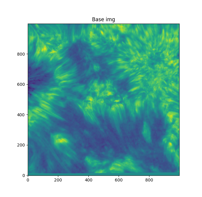
We need to bring out those individual fibular strands, and make them clearer. They're pretty indistinct as is, and blurry. If we sharpen the image with skimage's unsharp mask (radius=1, amt=4.0), we get something like this:

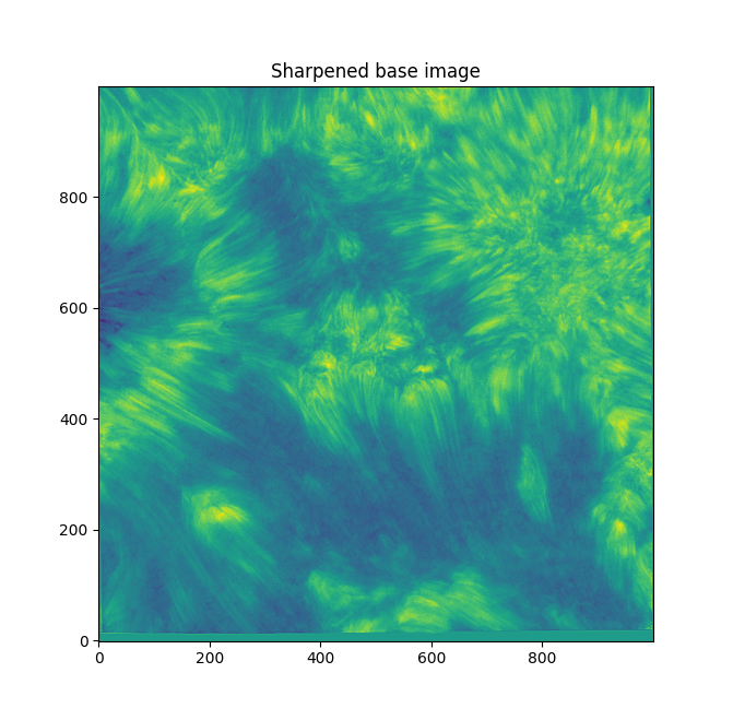
Better. Now - working on the entire image can get chaotic and force us to zoom in a lot. Let's focus on fibrils in a small sub-section - the bottom left has some distinct fibrils.

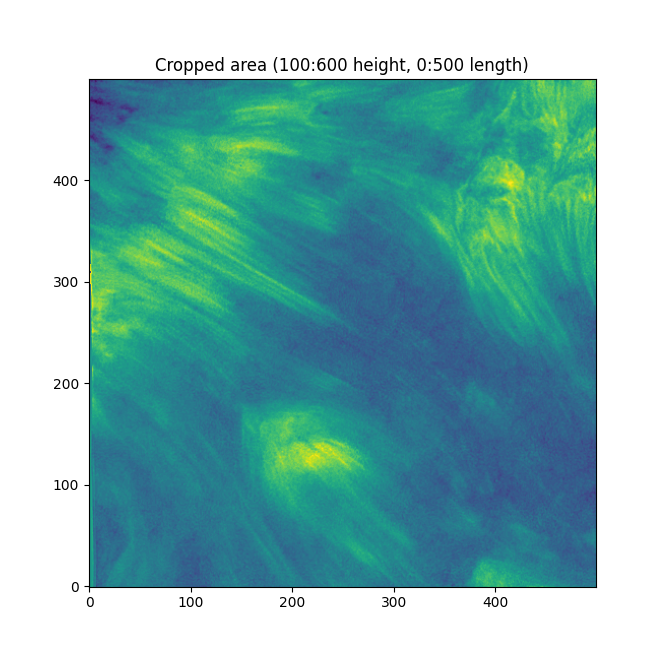
Now. We have a lot of background here - let's try some thresholding techniques. Otsu's method is an advanced technique for this - it'll look at the histogram of the image, look for two peaks, and then create a threshold between two threshold "peak groups". This GIF does a great job of visualizing it. I superimposed the original image to ensure Otsu was correctly measuring out sections.

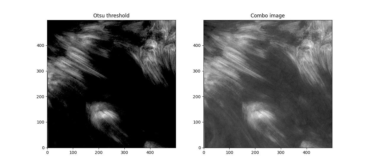
Otsu does an okay job at this, but some features are cut off. I subtracted a 0.05 offset to the threshold otsu found, which resulted in

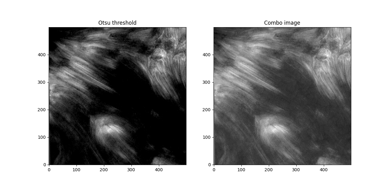
Better. This offset added some background noise - but we can deal with that later. Now, we've got some distinct fibrils - if we try out OCCULT on it,

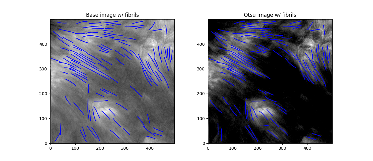
Similar results, but without a lot of the more indistinct fibrils that may blend into the background in low-seeing conditions. While it does remove some fibrils, I think the tradeoff in removing low-confidence fibrils is worthwhile.

Now, to try and make our fibrils a bit more distinct. skimage has an awesome script to test out the variety of segmentation functions available to skimage.

I'll probably go near-sighted just trying to make out these little images. But, of the results, I'm liking the look of both Hessians and the Meijering with sigma=1.

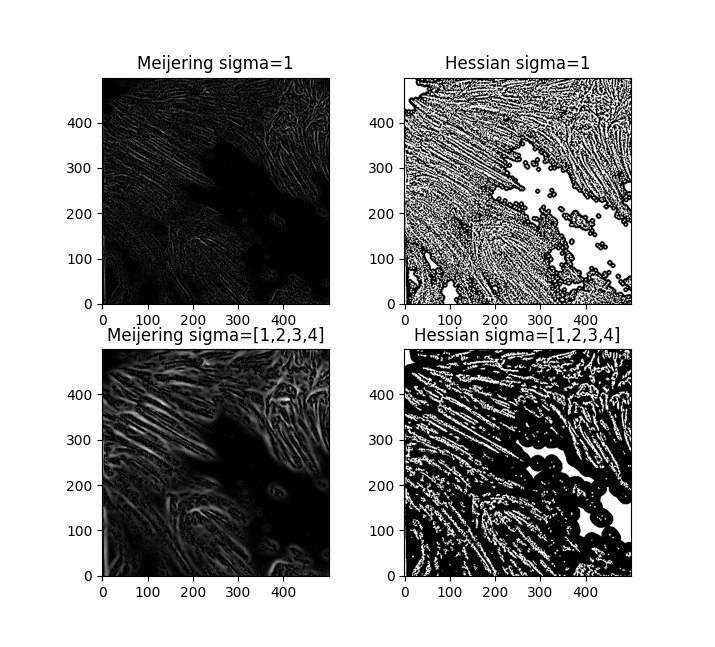
Let's go with the Hessian. Now - the Hessian matrix is a brilliant idea in image processing. If you've taken multivariable calculus or linear algebra before, you might remember it - mathematically, the Hessian can be represented as

$$\vec{H}_f = \begin{bmatrix} \frac{\delta I^2}{\delta x^2} & \frac{\delta I^2}{\delta x\delta y} \\ \frac{\delta I^2}{\delta y\delta x} & \frac{\delta I^2}{\delta y^2} \end{bmatrix}$$

In our context, this matrix describes the second order intensity variations around a given pixel. The eigenvalues of that Hessian matrix per pixel can then be used to evaluate the "local intensity curvature" - this article does a much better job of explaining it than I can.

We can deal with the large white blobs by just intersecting the image with the otsu tracing - leading to

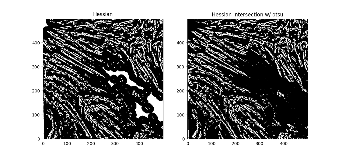
If we try out OCCULT-2 on this,

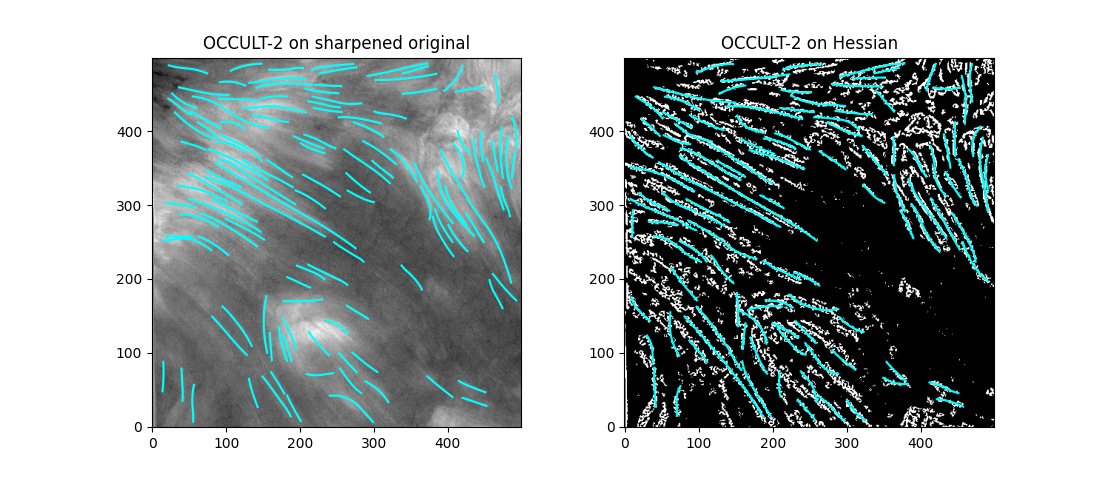
It's hard to say if it's better or worse. Many well-defined features are shared, some are lengthened, and some are gotten rid of entirely. Still - the entire goal of this tinkering was to reduce the impact of varied seeing conditions. If we try to compare the two timeseries now ...

Or, faster,

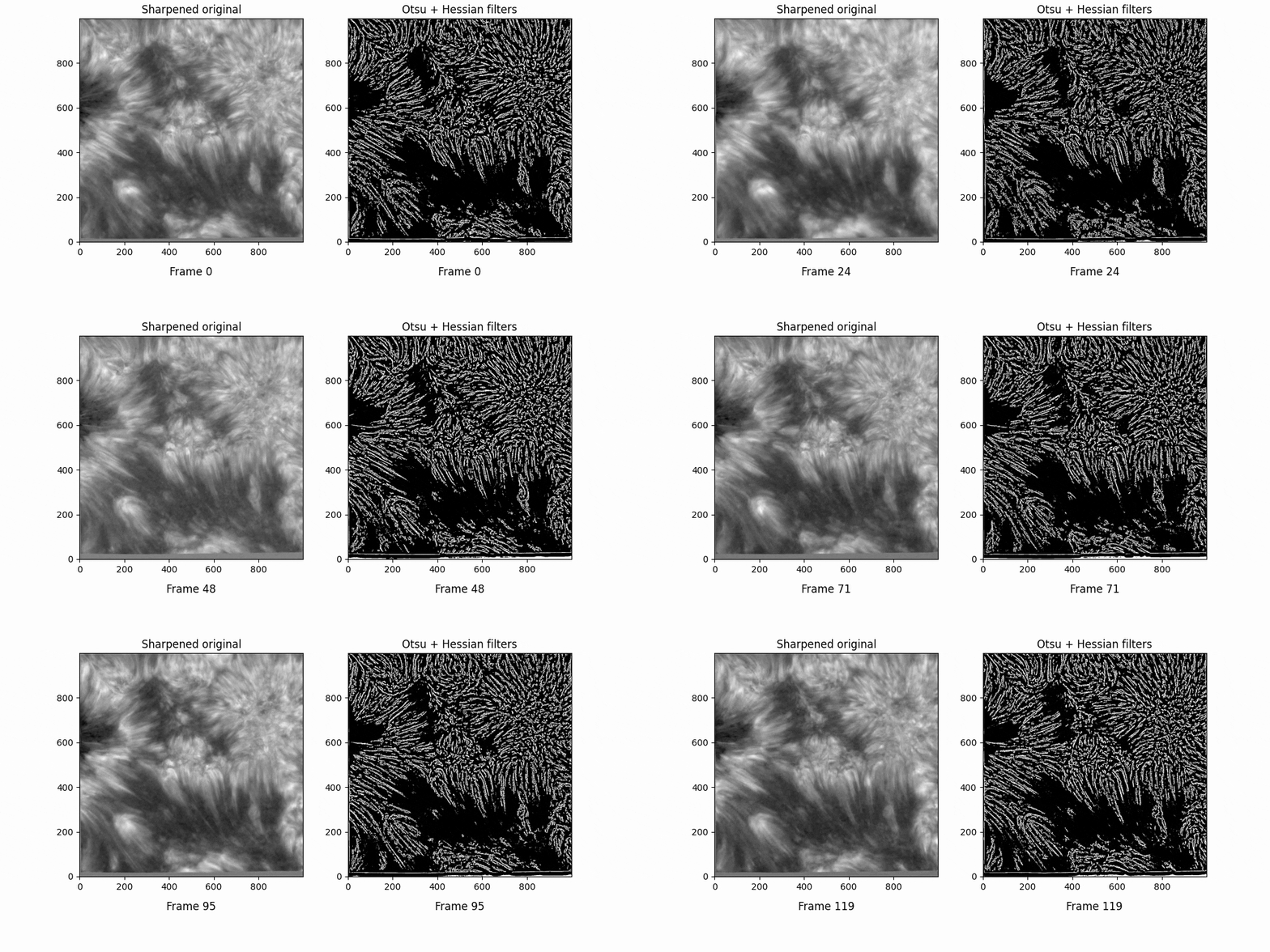
Graphing OCCULT-2 fibrils along this sequencee,

Faster,

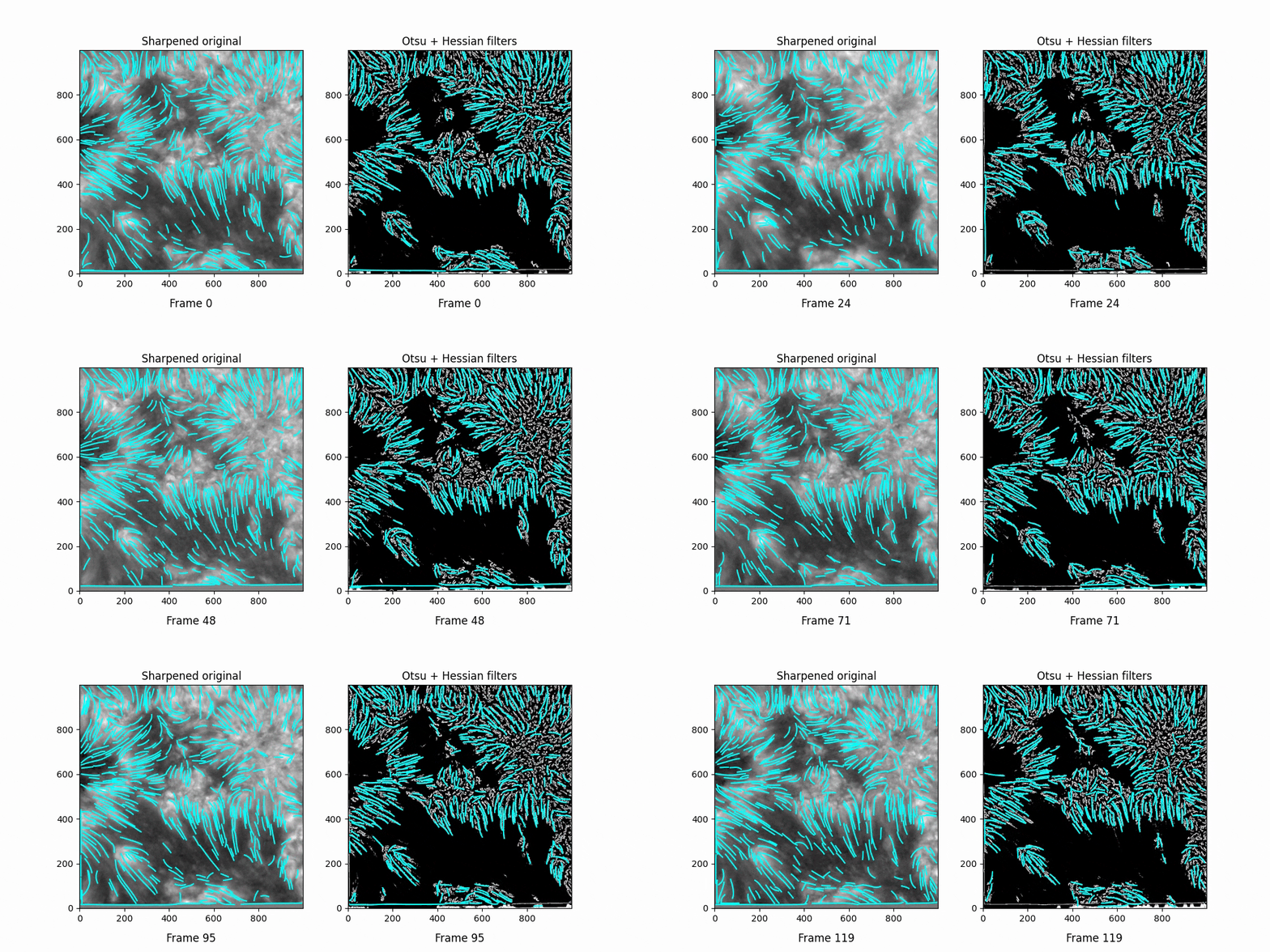
We see OCCULT recognizes many of the same fibrils and holds them relatively constant over time ... but many are extremely short lived, even where we can visually observe them still existing. In this scenario, it's likely OCCULT itself that is failing to recognize the existence of them.

This is ... okay. We could work with this. But, we're able to transform the image such that it has visibly consistent feature regions - having something more robustly able to detect these centerlines would be preferrable.

skimage segmentation

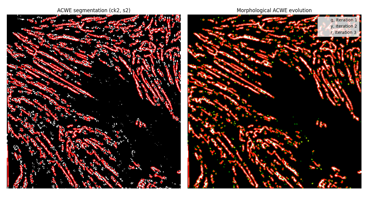
I played around with some of skimage's segmentation methods (of which there's many). I achieved some good results with our base Hessian image through the MorphACWE (implemented as the morphological Chan-Vese algorithm in skimage), resulting in

And with the find_contours method,

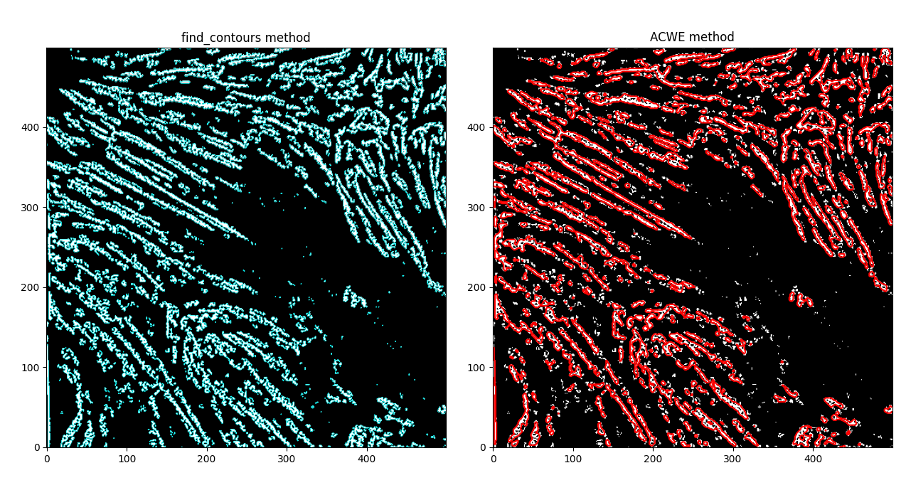
MorphACWE creates more "normalized" areas by virtue of doing some image transformations to smooth out regions - the contour method, by contrast, finds every area where the image intensity goes from 0 -> 1, and makes a polygon out of it.

I think we could achieve some good results by doing a contour evolution.

So, let's try to smooth the image out, "fattening" light regions. Let's try out a Gaussian first.

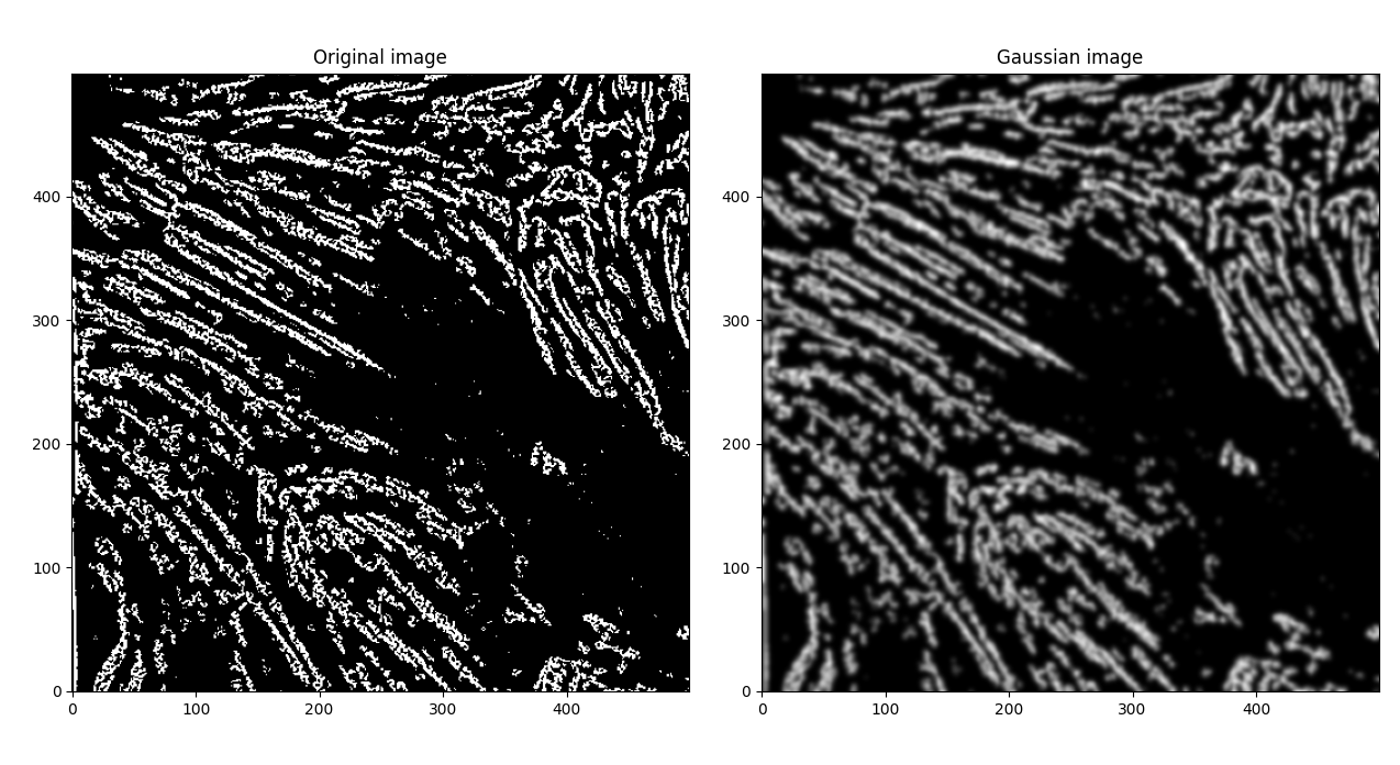
If we apply another Otsu filter to get back to a binary image,

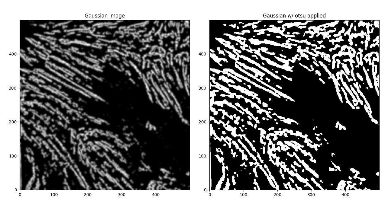
If we start to plot our contours now, we see

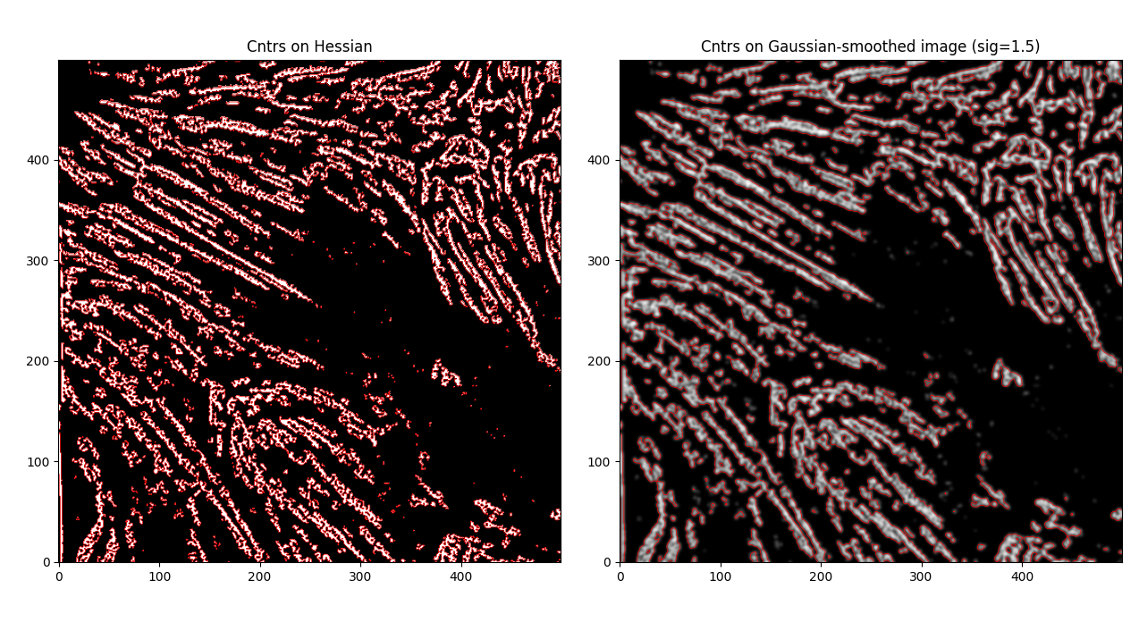
Much smoother, and some previously non-joined fibrils are now joined. However - this is an issue as well, as now we have some close distinct fibrils that are now joined together, which we don't necessarily want. That said - let's try to calculate some centerlines through these by using the label_centerlines library.

Note: Offstage, I've been really trying to bring out every single visually identifiable fibril, which I really just don't think is possible with an algorithmic approach. Neural networks might do a bit better. But still, we'll try to work with this Gaussian contours setup. I think we can come up with something good.

Okay. Label centerlines. This library is designed to work with shapely Polygons - and our find_contours function just returns lists of points in (x,y) format, so polygon conversion is nice and easy.

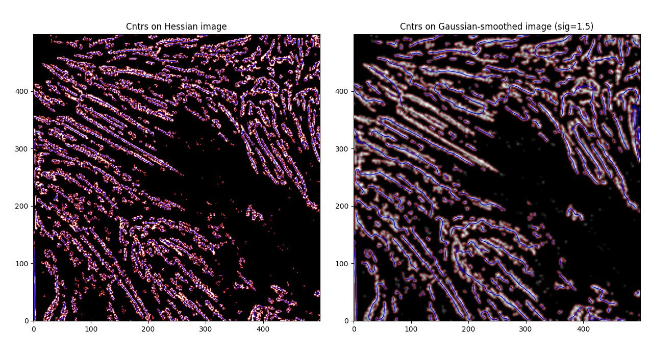
label_centerlines did exactly what we asked of it - but, there's some definite issues with unrelated features being joined (see left center) and some single features not being correctly joined (see bottom left).

We can try some morphological transforms to help with this. Dilations blow up light areas, while erosions reduce light areas. Focusing on the bottom left $(110\times90)$ px region,

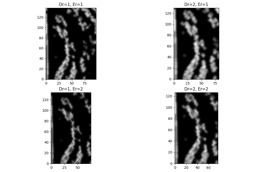
Great! Except, now ...

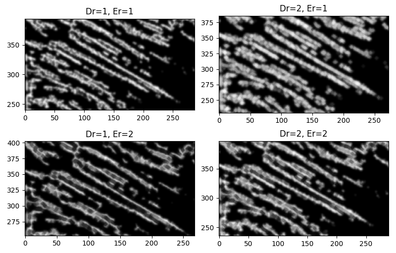
I know. I know! I ought to have expected it. Dilations will close small spaces, and will not distinguish between spaces between disconnected fibrils and separate features.

Okay.

Let's think. Easiest to address - first - our features are pretty grainy, and there's a lot of small holes everywhere. Let's try dealing with that first.

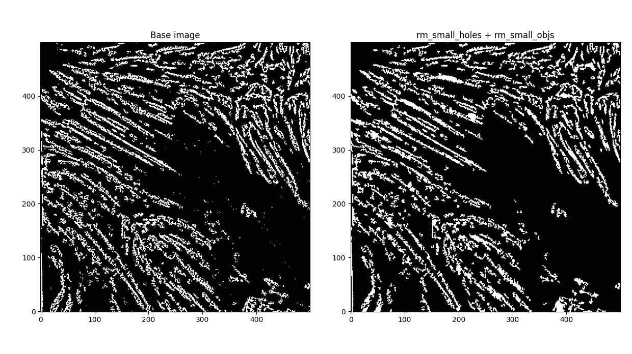
Dilated (square=1), filled small holes (s=64), removed small objects (s=10) (Note: any larger small object size removed parts of fibrils).

Now.

What if we did a polyfit on larger polygons? Take an average over all polygon sizes; those that are greater than the average, do a polyfit, add smaller polygons to them.

This is an interesting idea. Let's try it.

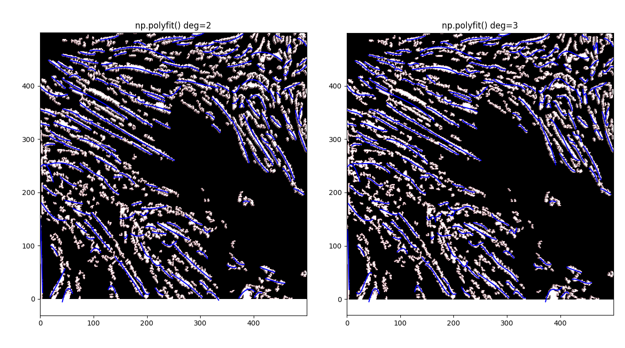
Nice! Cool thought. Still - the broken-up-ness of individual features is making the lines curly and go all over the place. I did some further reading into skimage's filters - and there are some that could help with this, such as the Meijering (I know, I dismissed it earlier in favor of the Hessian - but what if we did both?)

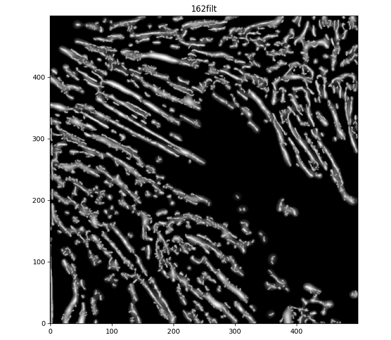
sigma=(1,7,1). Adding a median filter to make things a bit less contrasty, and thresholding to disconnect some unrelated features, we get

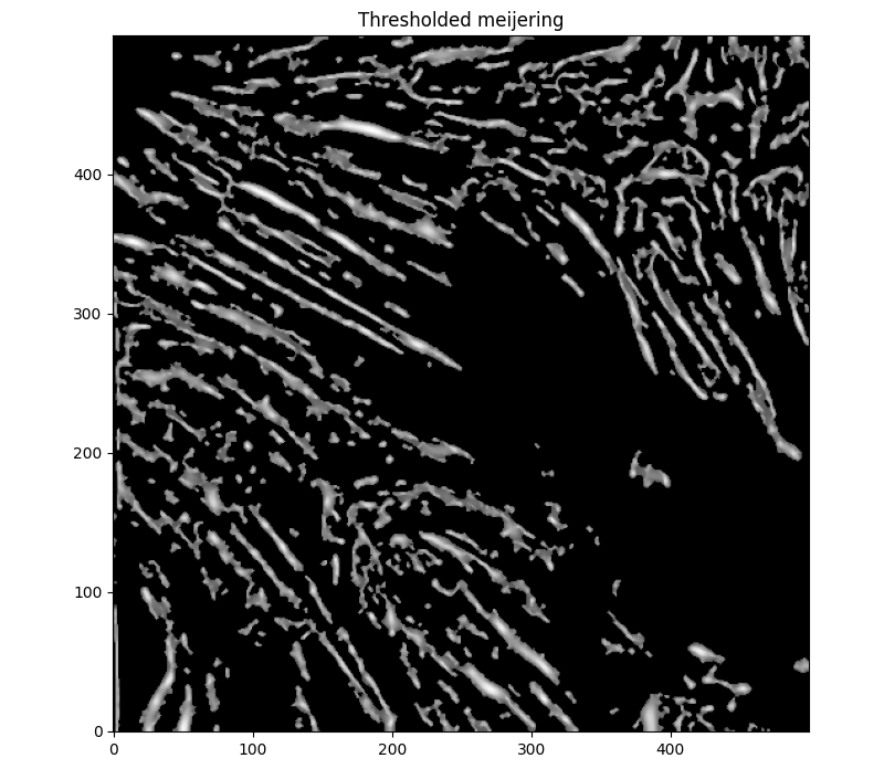
This looks .. okay. Pretty jagged as a whole. Still, I did more reading on models other than threshold-based contouring to match edges, and did further reading into Morphological ACWE. The old github page on Morphsnakes has some pretty sweet animations, too -

Which made me quite interested in trying them out once more, as they could be used to deal with this jaggedness.

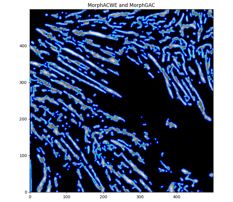
ACWE (cyan) with checkerboard set s=4 and i=10, GAC (blue) with thresholded version of Meijering as level set (t=0.3), i=1, b=0.

Better results from ACWE so far.

---

Another day, another night of background thoughts. I'm worried the amount of processing we've already done will lead to seeing affecting the ability for morphsnakes to ID fibrils significantly. Still - we'll address that soon. MorphACWE has done a great job with only i=10 - but, I think we can make it do better. Things to try today:

1. Create level set from thresh (better)
2. Create level set out of local mins and maxes
3. Try local thresholding following initial otsu to better define fibrils
4. Visualize evolution of morphsnakes in all scenarios using morphsnake callback

Let's try out some different level sets with MorphGAC.

1. base=filt1, init_ls = filt1>0.3
2. base=inv_gauss_grad, init_ls=filt1>0.3
3. base=filt1, init_ls=extrema.local_maxima

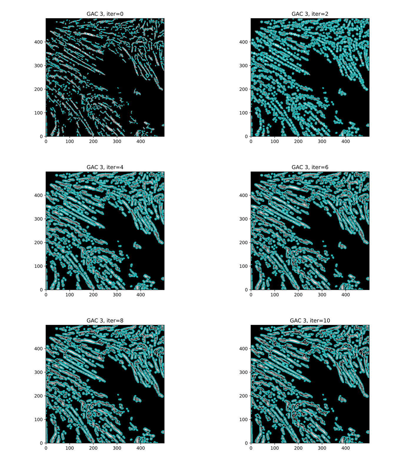
And trying ACWE (base=(filt1[filt1 < 0.33] = 0))

1. init_ls = filt1>0.3
2. init_ls = checkerboard_level_set s=2
3. init_ls = morphology.extrema.local_maxima

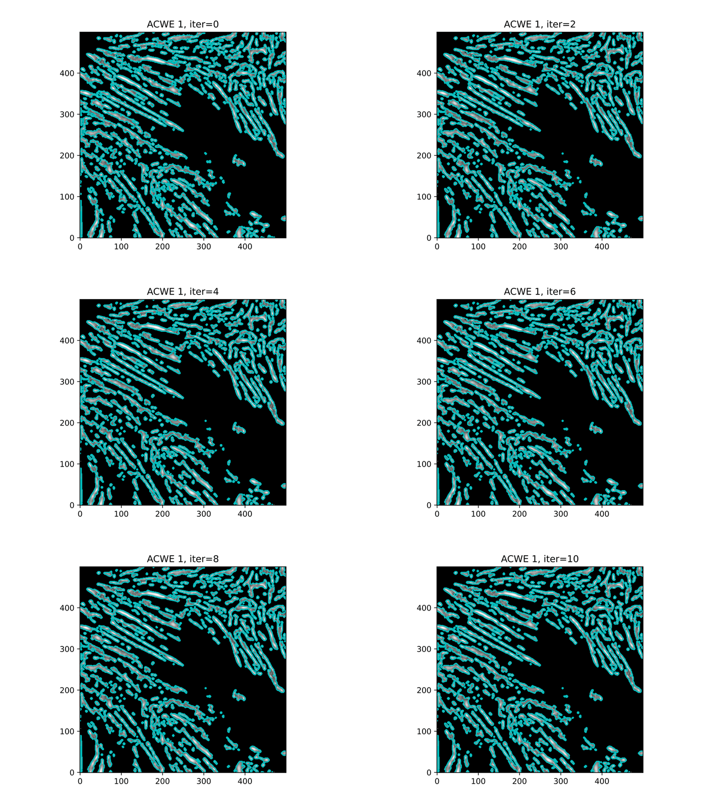
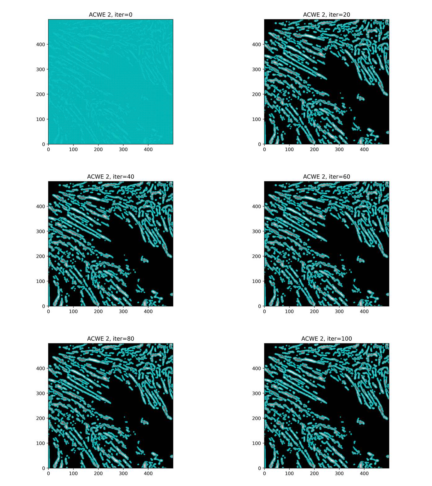
GAC 2 and ACWE 2 are best so far; though I intend on playing around with both types later. If we can get a more dense seed pattern, ACWE 3 yields promising results.

Now, changes in seeing. This isn't a bad issue - except - for issues that become apparent such as in GAC 3, where features above and below combine. This will happen - so we need to find a way to prevent 2+ fibrils from "merging" into one due to closeness.

Is there a way to quantify the linearity of polygons? Or ... can we divide a polygon into two maximum-area subpolygons? ... Some brief reading online leads me to believe this a challenging problem.

Which, circles back to optimizing ACWE further. If we can encourage a style similar to ACWE3, except with more seed points ... let's try to find more seed points. Or, smooth further?

---

Unfortunately, further optimization of the Hessian yielded little improvement. The main issue is the gap between some fibrils is equal to the gap along fibrils - so any work to close these gaps along also causes gaps between to be closed, and active contouring isn't designed to do any distinguishing here.

Also of note - the fibrils are barely distinguishable from one another in the initial image itself - so further optimization here might not do much ... unless ... we increase the offset in the otsu thresholding even further ... no, that just results in more noise, unfortunately. If we try Sauvola thresholding and the local otsu as an alternative to the global otsu,

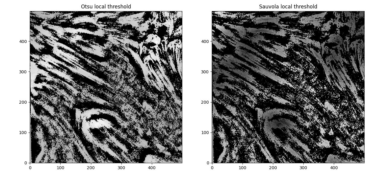
(window_size=45 in both cases). The Hessians then look like

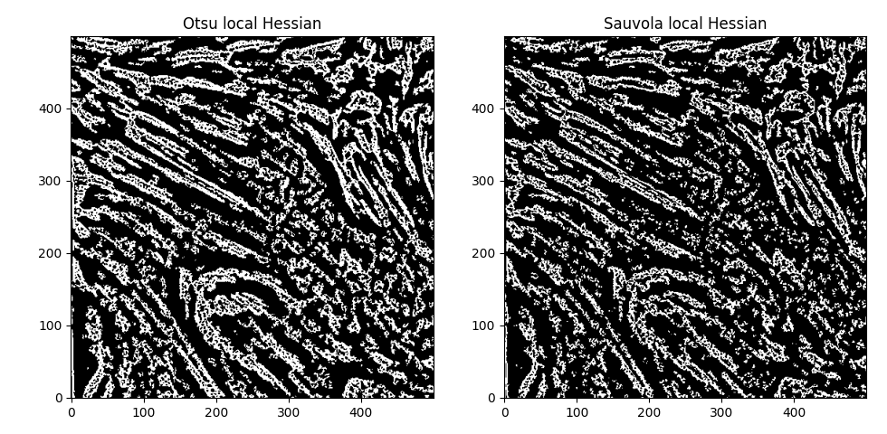
Interesting. Hmm. Comparing the global and local thresholding for Otsu,

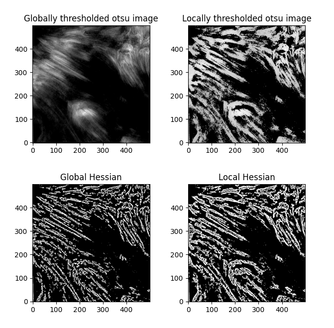
with a corresponding Meijering for the local sigmas=range(1,5,1) of

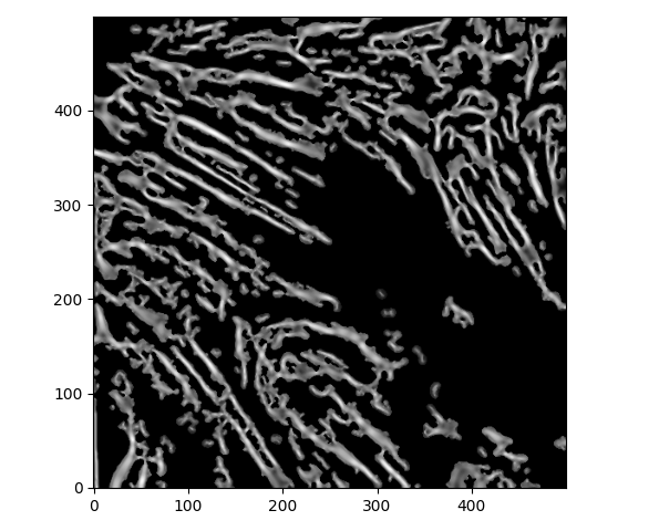
... I don't think any amount of local filtering is going to help us here. The only thing that comes to mind is that we have to split large polygons into sub-polygons depending on their curvature.

Ugh.

Fine.

---

Tracing out centerlines without our curvature segmentation and parameters max_paths=10, smooth_sigma=13, we find

Not the best - there's a lot of curves that are much too curvy. We could ignore these by filtering out high-curvature polygons/centerlines, but let's try out our fancy new curvature segmentation algorithm first.

Let's try segmentation with our default parameters.

Fantastic! Already we're seeing some marked difference in identified fibrils. If we loosen the parameters a bit to accomodate for smaller and tighter polygons, (min_area=150, percent_thresh=0.2), and then an upper limit by loosening the threshold a bit (min_area=150, percent_thresh=0.3),

The tighter version (0.2) has a lot more cohesivity of polygons than the looser version, particularly visible on the lower "C" curve toward the base of the image center. Let's try it out and trace out centerlines in all polygons of area > 150, using both the get_centerlines library and np.polyfit(deg=2).

Looking really good. get_centerlines conforms to the polygons a lot better, while polyfit generates much smoother lines - let's take another look at the OG image to see which we want.

I think the polyfit method works better, to be honest - few of our features have visible high curvature, however the contrast isn't good enough to definitively say one way or the other.

---

Note: This method ignores a lot of fibrils, in favor of "fibril regions". I believe we can either focus on bringing out every single fibril and having a ton of noise, or bringing out just a few "fibular groups" and having them be relatively well-defined over several images.

These centerlines therefore should be representative of the evolution of fibular groups rather than fibrils themselves. It's an unideal result - but the lack of consistent seeing and the fact that our fibrils operate right at the resolution limit of the imaging camera may make this an unavoidable dichotomy.

---

Note 2: As a todo, let's try matching together fibrils that are just barely separated (such as around x=50, y=200) in the polylines centerlines.

---

Either later tonight or tomorrow I'll look at how these centerlines evolve over the full timeseries, and compare it with our OCCULT evolution. Pending further optimization of our curvature segmentation parameters depending on the results of the timeseries evolution, it's almost July and I'll need to call this good in favor of working on the paper + getting results.

This work should be considered, for now, the best I've been able to do with the current resolution limit. Once updated data with a higher resolution limit from DKIST becomes available, I'd like to revisit this.

---

With the original slice, the execution time of our demo script is:

Executed in    7.11 secs    fish           external
   usr time   10.18 secs  568.00 micros   10.18 secs

With the full image, this becomes

Executed in   78.39 secs    fish           external
   usr time   32.99 secs  299.00 micros   32.99 secs

Runtime triples, but is with the full curvature segmentation in place. For the full 120 image sequence assuming similar quantity of fibrils on average, the runtime will be about 3840 seconds (just over an hour).

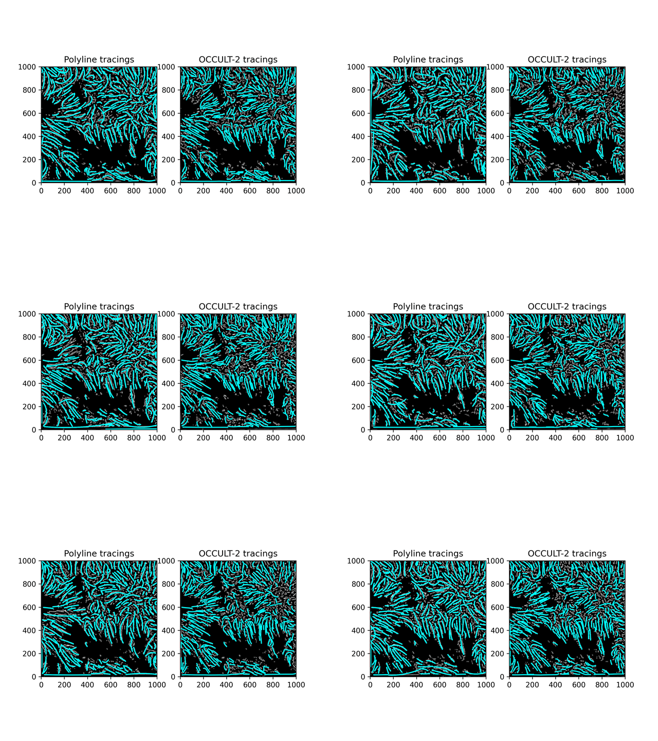
Fibrils don't disappear as much as in the OCCULT-2 version - but they do get disconnected and disjointed when seeing is bad. To help reduce noise, let's first add another minimum area filter (don't calculate polylines for less than 300 pixels area) and only run the script for a period of good seeing (62-87).

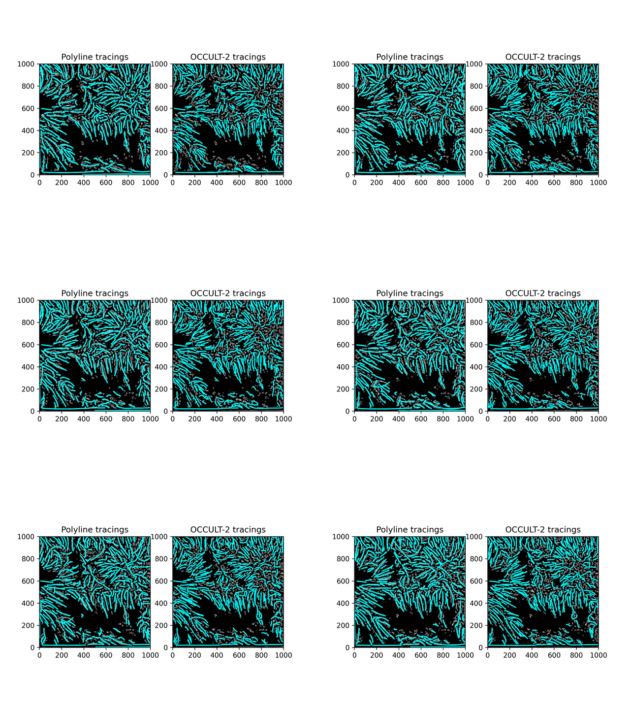
Similar results. While this isn't what was hoped for - it is an alternate method to OCCULT-2 that we can use. Let's characterize them and continue.